Small introduction

In the field of computational quantum chemistry, scientists model molecules using foundational physical models like density functional theory. These methods are electronic, which according to our good pal of recent popularity Oppenheimer, is only half the story. Nuclear contributions to the molecular wavefunction include vibrations of the atoms within the molecule. The solution to foundationally accurate molecular simulations is as simple as computing the electronic energies of all possible atomic configurations, and assessing the likelihood of finding the molecule in each configuration. The problem is that there’s no computationally tractable way to visit every single configuration and run a computation. If this sounds like the setup to a Bayesian problem, you’re paying attention.

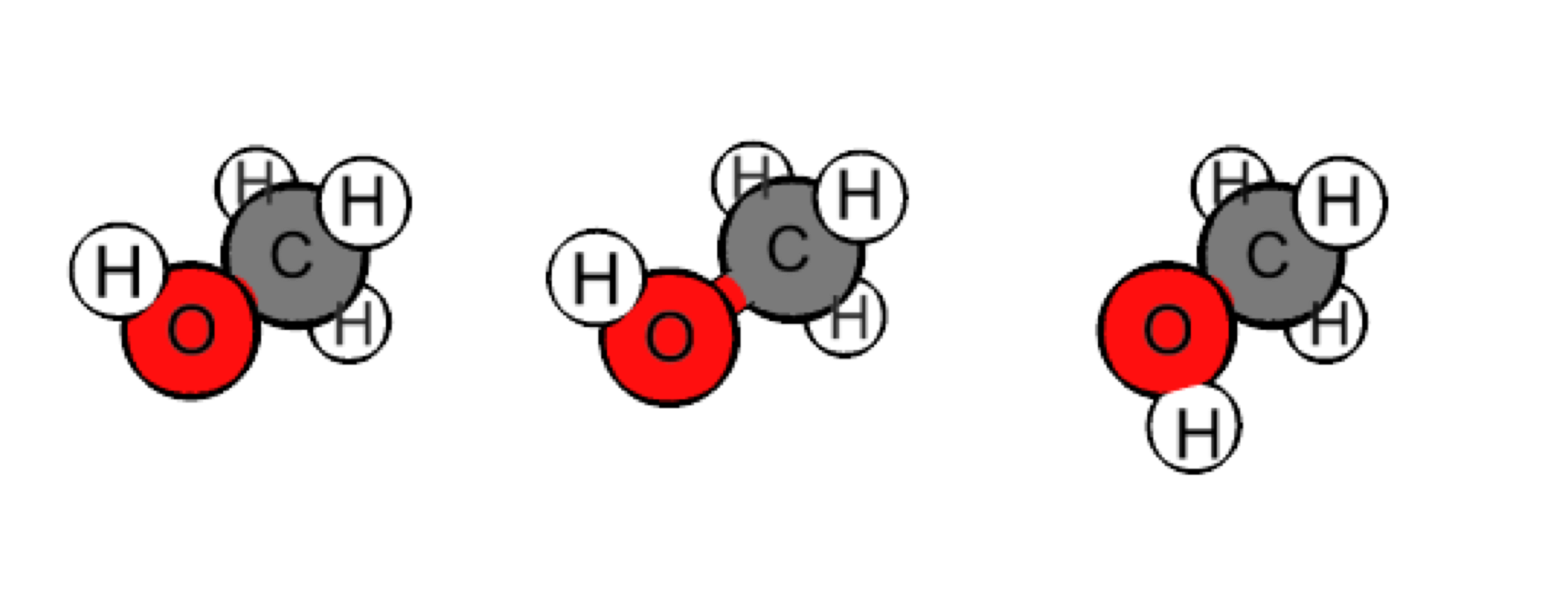
Take a look at methanol, six atoms, and 6 $\times$ 3 = 18 input variables, one for each Cartesian coordinate. Each configuration vector $x_j \in \mathbf{R}^{18}$ is a single input to the a ab initio predictor, $V(x_j)$. $x$ is realistically constrained to certain spatial values – molecules stay together after all. These can be represented as stretches, bends, and rotations within the molecule, like this:

Even with constraints on the internal “relative” positions of the atoms w.r.t. each other (i.e. feature engineering a.k.a. coordinate transformation a.k.a. internal coordinates), visiting every possible input $x$ and computing the energy is prohibitively expensive, even when parallelized.

Don’t forget, in silico quantum mechanics simulation requires constructing and diagonalizing a matrix in a finite basis. Even for small molecules like methane, this is severely limited by memory and computation cost.

Further complicating things, classical simulations such as molecular dynamics (glorified Newtonian mechanics) are not actually foundational because molecules are quantum mechanical. The consequences are an inaccurate model (validated on data from laboratory measurements/observations).

Many assumptions simplify the model at the cost of some degree of technical accuracy. Take, for example, the assumption that the potential energy of molecule $V$ is linear with each motion (out of $3N$).

V(\vb{x}) \,=\, \sum_{i=1}^{3N} V_i(x_i)

Then one needs to train just $3N$ models and add their result, where $N$ is the size of the molecule in atoms.

The choice of model for $V_i$ is critical but surprisingly intuitive. With each $V_i$ explaining a motion, we can fit synthetic spatial data for each motion to a basis function regression model. This is the subject of previous posts for polynomial, Fourier, spherical harmonics, and symmetric top bases. How we obtain quantum expected values is explained in these posts.

This works until it doesn’t. In fact, correlations should be expected under certain circumstances, like a molecule whose moment of inertia changes with configuration.

P(\vb{x}) \,=\, \prod_{i=1}^{3N} P_i(x_i)

This implies that $V(x')$ can be modeled through a linear response model, so that each component can be evaluated independently:

Then we only need to solve 1-D functions of each component using basis function regression techniques, and independently solve each 1-D Schrödinger equation using eigendecomposition methods.

$$-\frac{1}{2} \nabla^2 \Phi_i (X_k) + v_k (X_k) \,=\, E_i \Phi_i(X_k)$$

We can compute each marginal probability density function $P(X_k)$ using the squared probability amplitude, which is the pdf for $X_k$ conditioned on $\mathscr{E}$:

$$P(X_k=x \,|\,\mathscr{E}=E_i) \,=\, \left| \Phi_i^*({x})\Phi_i({x}) \right|$$

$$P(X_k) \,=\,\sum_i \, P(X_k \,|\,\mathscr{E}=E_i) \, P(\mathscr{E}=E_i)$$

The motivation for doing this is that we can now be much more intelligent about how we construct our data table. Since we only want to expend computational power for a feasible number of data, we can directly sample the expected distribution of $X$ to increase our confidence that the expected values computed from the data are representative of the “population” means.