Quantum ML models for periodic, spherical, and 3-D rotational data
In the a previous post about quantum variational inference on polynomial models, I showed how you can infer expectation values & uncertainties of discrete random variables by regressing log-probability data () and finding the eigenvalues of the equation
using variational inference. But very few data can be reliably fit to a polynomial. Like, for example, periodic data such as daily power usage, bioavailability medication taken daily, or a chemical bond rotation. Or like latitudinal and longitudinal data, e.g. positions on a globe or the orientation of a linear molecule. Or, even more complicated, like latitudinal and longitudinal AND periodic data – like 3-D pose detection data or the orientation of a non-linear molecule.
This post is about how to train a machine to learn these more complicated cases:
- Regression to a Fourier series expansion for N-D periodic data (),
- Regression to a spherical harmonics expansion for spherical data (), and
- Regression to a Wigner D-matrix series expansion for 3-D rotational data ().
Let’s do some Quantum ML.
Regression & Quantum Variational Inference on a Fourier Expansion
If we have a function of the periodic input data , we can find a representation of by taking a linear combination of sines and cosines (a Fourier series)
class FourierSeries(torch.nn.Module):
    """
    Trainable 2*pi-periodic Fourier series
    """
    def __init__(self, order=8):
        super().__init__()
        self.c = torch.nn.Parameter(torch.zeros(1 + 2*order), requires_grad=True)

    def forward(self, x):
        y = 0.
        for n,c in enumerate(self.c):
            y += c*self._fourier_fn(x, n)
        return y

    def _fourier_fn(self, x, n):
        if n == 0:
            # zero / constant
            return np.power(2*np.pi, -0.5)*torch.ones_like(x)
        elif n % 2:
            # odd n / cos
            return np.power(np.pi, -0.5)*torch.cos(0.5*(n+1)*x)
        else:
            # even n / sin
            return np.power(np.pi, -0.5)*torch.sin(0.5*n*x)
Conveniently, we can also use these as basis functions for a quantum model, since we know
Confused? See previous post. In code, we can define a Fourier regression model similar to the polynomial regression model as so
class Ring(QuantumBasis):
    def __init__(self, order):
        super().__init__(order)

    def potential(self, x):
        return 0 * x

    def basis_fn(self, x, n):
        if n == 0:
            # zero / constant
            return np.power(2*np.pi, -0.5)*torch.ones_like(x)
        elif n % 2:
            # odd n / cos
            return np.power(np.pi, -0.5)*torch.cos(0.5*(n+1)*x)
        else:
            # even n / sin
            return np.power(np.pi, -0.5)*torch.sin(0.5*n*x)

    @staticmethod
    def H_basis(order):
        return 0.5*torch.diag(torch.cat([torch.zeros(1),
                                         torch.arange(1, order+1).repeat_interleave(2)]).square())
So similar to the previous post, here’s the quantum ring model for any periodic feature and its response :
class FourierQModel(nn.Module, Ring):
    def __init__(self, potential_model, dim, trapz_grid=200):
        super().__init__()
        super(Ring, self).__init__(dim)
        self._potential = potential_model
        self.loss_fn = F.mse_loss
        self._x = torch.linspace(0, 2*np.pi, trapz_grind)

    def forward(self, x):
        return self._potential(x)

    def potential(self, x):
        return self(x)

    @torch.no_grad()
    def update(self):
        H = self.H_base.clone()
        x = self._x
        for m in range(H.shape[1]):
            for n in range(m, H.shape[0]):
                y = self.basis_fn(x, m) * self.potential(x) * self.basis_fn(x, n)
                elem = torch.trapz(y, x)
                H[m, n] += elem
                H[n, m] += elem
        self.H_matrix = H
Here’s an interesting potential
xdata = torch.linspace(-np.pi, np.pi, 100)
V_ring = lambda x: 15*torch.heaviside(torch.cos(x-np.pi), torch.ones(1))
ydata = V_ring(xdata)
Here is how we learn the quanta & compute the thermodynamic metrics…
potential = FourierSeries(25)
qmodel = FourierQModel(potential, 25)
cost = torch.nn.MSELoss()
optim = torch.optim.Adam(qmodel.parameters(), lr=1e-2)
for step in range(50):
    for x,y in zip(xdata, ydata):
        optim.zero_grad()
        pred = qmodel(x)
        loss = cost(pred, y)
        loss.backward()
        optim.step()
    qmodel.update()
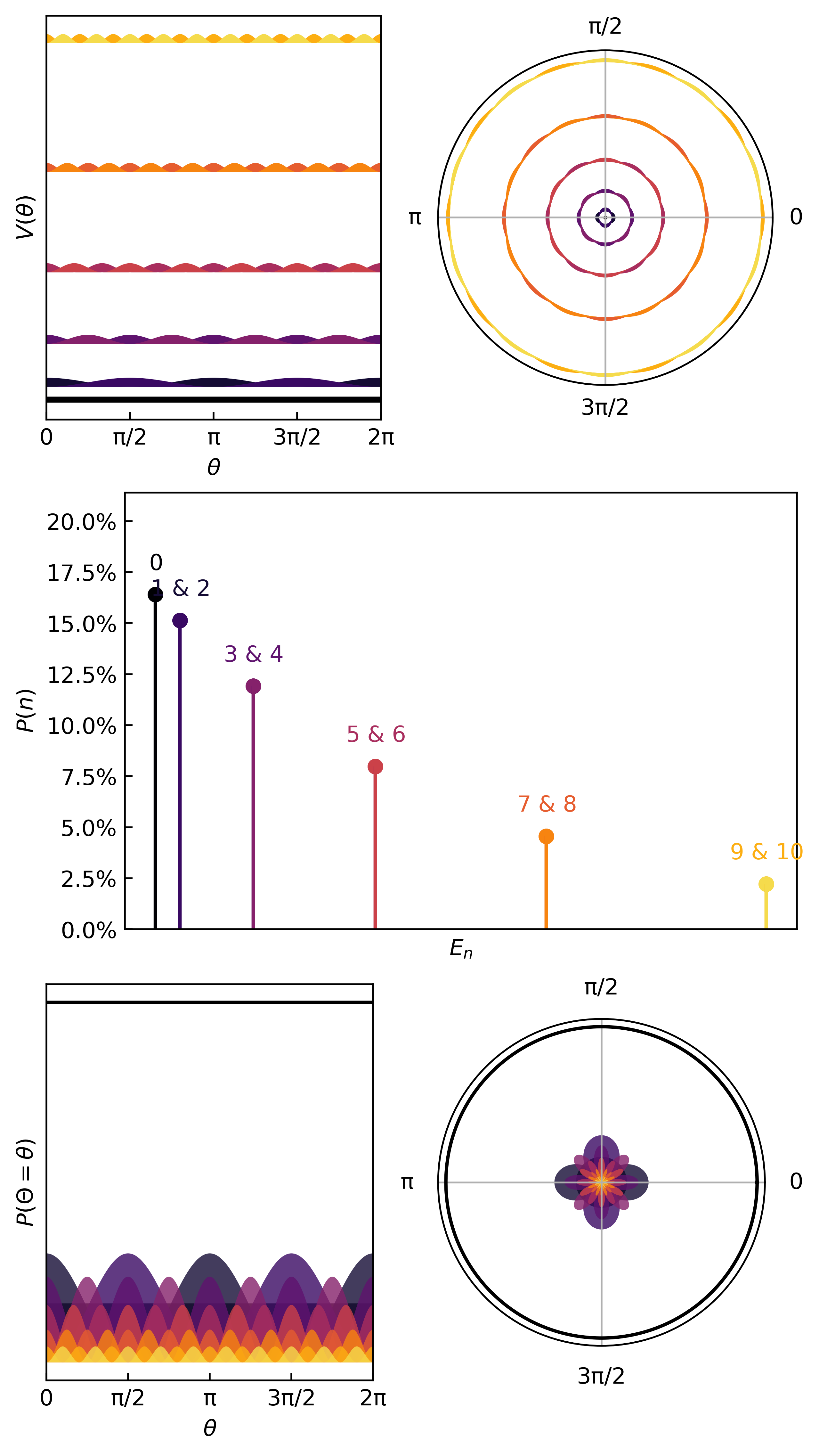
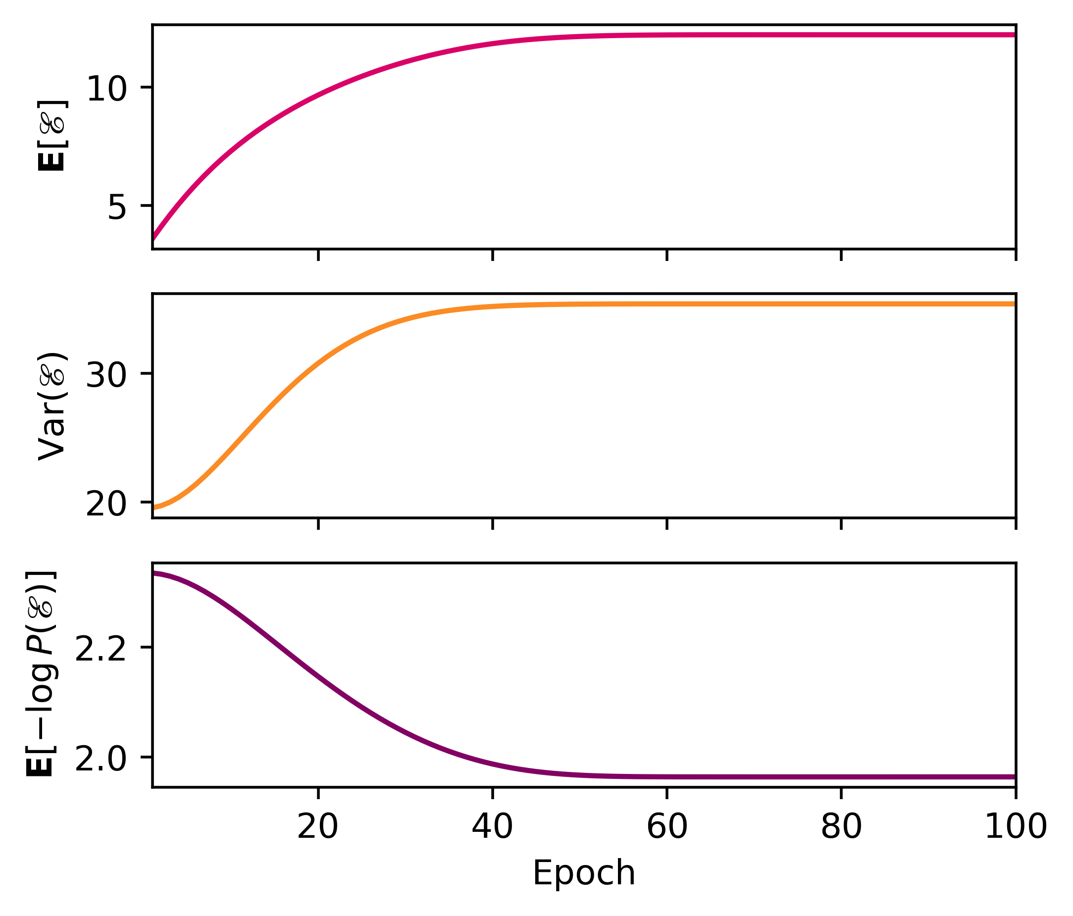
And here are the first few quanta & probabilities.
The statistics (mean, variance, entropy) come from the same quantum statistical mechanics protocol as before.
Regression on a Spherical Harmonics Expansion
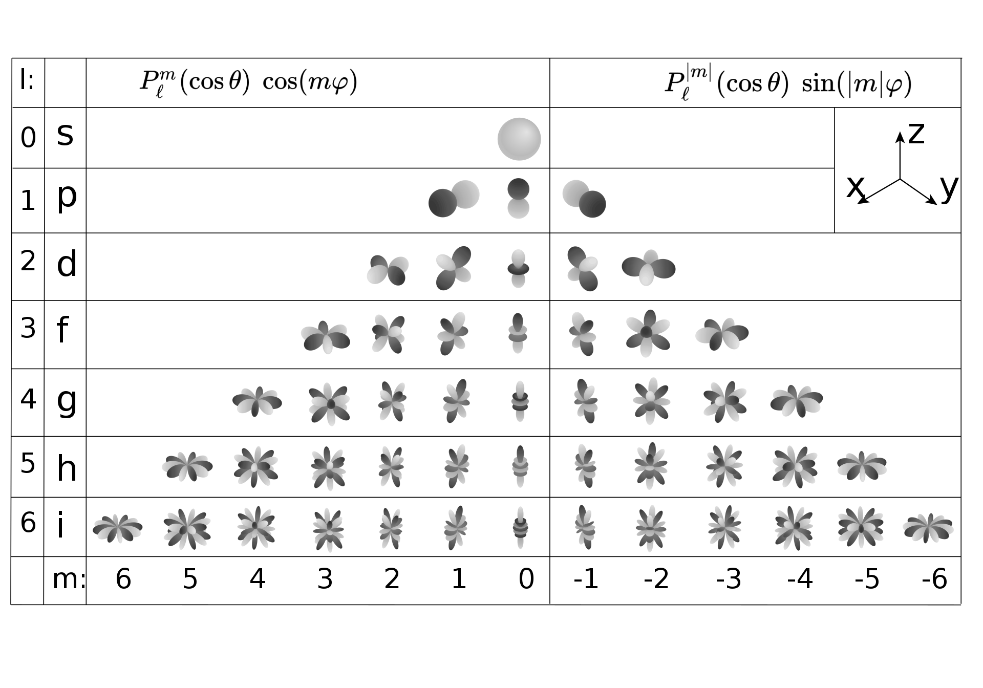
The process of modeling spherical data is basically the same, except using spherical harmonic functions . Unlike a 1-D Fourier series, however, spherical data is parameterized in two dimensions, latitude and longitude , and thus needs two integers (quantum numbers) encoding its coefficients,
where the functions are the Legendre polynomials. These can be visualized in the following table, courtesy of Wikipedia:
Despite the daunting look of these equations, it’s actually quite easy to build a linear regression model using already-existing functions from modules like scipy.special;
from scipy.special import sph_harm as Y

def spherical_fit(xpts, ypts, max_iter=20, tol=0.05):
    lmax = 1
    prevR2 = 0
To demonstrate how this works, I’ll use actual data that I really used in one of my projects to describe the orientation of a molecule, which is parameterized by three features: latitude , longitude , and polar rotation . Here is a useful image for visualizing this concept:
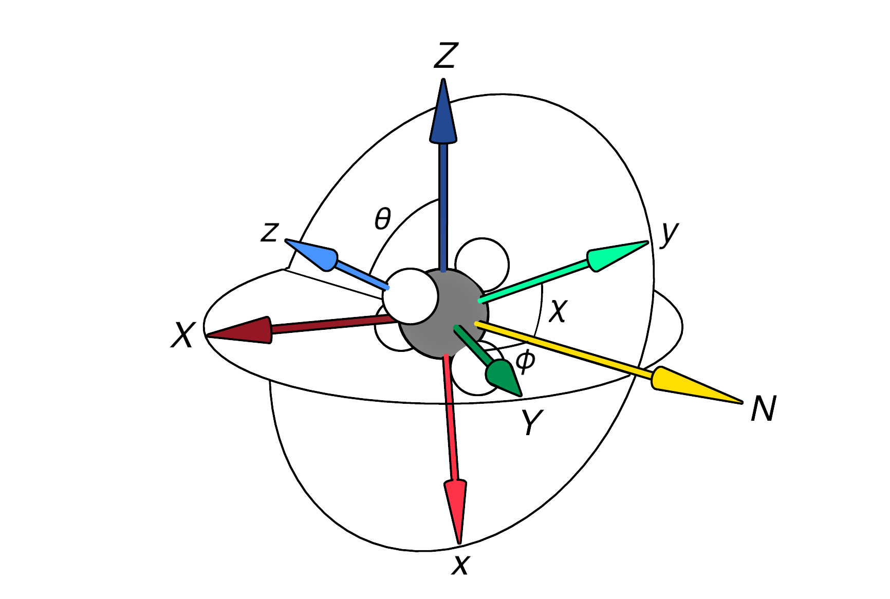
To draw a parallel to more common iterations of this kind of dataset, we can think of the data as representing global coordinates (latitudes and longitudes on Earth) with yearly, monthly, or daily periodicity encoded by . With that in mind, let’s make a model that assumes the latitudes and longitudes at an instant in time, say = 0.0:
>>> df = pd.read_csv('/path/to/wigner_data.csv')    # Read in the "Wigner" data
>>> sph_df = df[df['X3'] == 0.00]                   # Select only χ=0 data
>>> sample_x = np.array([np.array(sph_df.X1), np.array(sph_df.X2)]).T
>>> sample_y = np.array(sph_df.Y)
>>> coeffs, fit_fn = spherical_fit(sample_x, sample_y)  # fit the data
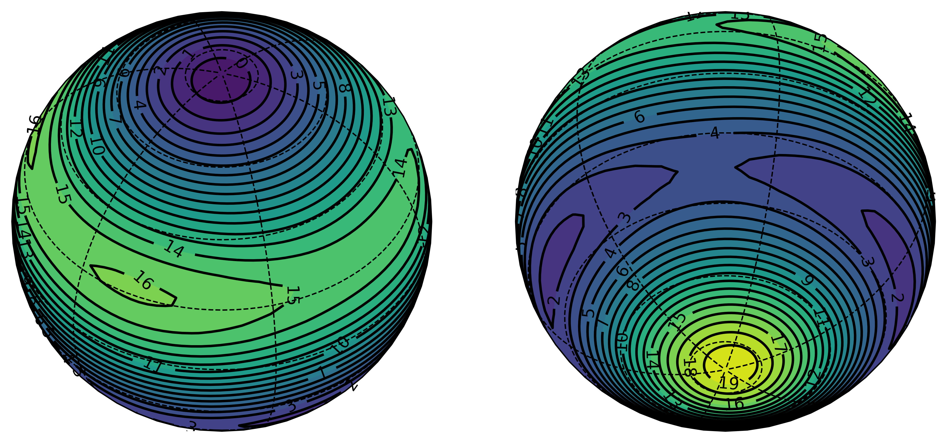
With spherical data, the result of the regression can be difficult to visualize, since it requires either mapping a projection of a sphere or simultaneously viewing podal and antipodal perspectives of a globe. Both of these options are luckily available when working with global data with a module called cartopy, and we can easily adapt them for our model.
import matplotlib.pyplot as plt
import cartopy.crs as ccrs
import cartopy.feature as cfeature

def generate_plottable_data(fn, shape=(73, 135)):
    nlats, nlons = shape
    lats = np.linspace(-np.pi/2, np.pi/2, nlats)
    lons = np.linspace(0, 2 * np.pi, nlons)
    lons, lats = np.meshgrid(lons, lats)
    # lat . = θ from π -> -π
    # long.  = φ from 0 -> 2π
    # f  = f(θ,φ)
    data = fn(lats+np.pi/2, lons) # latitude vs polar angle conventions
    lats = np.rad2deg(lats)
    lons = np.rad2deg(lons)
    return lons, lats, data

def spherical_plot(lons, lats, data):
    # Some parameters:
    PHI, THETA = 45,45      # Viewing perspective angles
    lvls = np.arange(-2,22) # This is data-specific, not general
    cmap = 'viridis'        # Nice colors

    fig = plt.figure(figsize=(10,10))
    ax1 = fig.add_subplot(121, projection=ccrs.Orthographic(PHI, THETA))
    ax2 = fig.add_subplot(122, projection=ccrs.Orthographic(PHI-180, -THETA))
    ax1.gridlines(color='black', linestyle='--')
    ax2.gridlines(color='black', linestyle='--')
    ax1.set_global()
    ax2.set_global()

    # Plot contours and countor lines, with labels, on BOTH plots
    filled_c1 = ax1.contourf(lons, lats, data,
                transform=ccrs.RotatedPole(pole_latitude=-90, pole_longitude=50),
                cmap=cmap, levels=lvls)
    line_c1 = ax1.contour(lons, lats, data,
                transform=ccrs.RotatedPole(pole_latitude=-90, pole_longitude=50),
                colors=['black'], levels=filled_c.levels)
    ax1.clabel(
            line_c1,  # Typically best results when labelling line contours.
            colors=['black'],
            manual=False,  # Automatic placement vs manual placement.
            inline=True,  # Cut the line where the label will be placed.
            fmt=' {:.0f} '.format,  # Labes as integers, with some extra space.
        )
    filled_c2 = ax2.contourf(lons, lats, data,
                transform=ccrs.RotatedPole(pole_latitude=-90, pole_longitude=50),
                           cmap=cmap, levels=lvls)
    line_c2 = ax2.contour(lons, lats, data,
                transform=ccrs.RotatedPole(pole_latitude=-90, pole_longitude=50),
                colors=['black'], levels=filled_c2.levels)
    ax2.clabel(
            line_c2,  # Typically best results when labelling line contours.
            colors=['black'],
            manual=False,  # Automatic placement vs manual placement.
            inline=True,  # Cut the line where the label will be placed.
            fmt=' {:.0f} '.format,  # Labes as integers, with some extra space.
        )
>>> lons,lats,data = generate_plottable_sph_data(fit_fn)
>>> spherical_plot(lons,lats,data)
Running this code, we have a nice representation of the spherical harmonics regression to an > 95%. Given any latitude and longitude, we can predict the value of our response variable given only the data at = 0.