Uncertainty is a fundamental of every day life – and not just in that we don’t know who’s gonna win the next election, or whether it will rain, or how long until the next bus comes. I mean that down to the atomic level, it’s impossible to pinpoint a single molecule, let alone an atom. As in the non-quantum world, probability theory helps explain the uncertainty – probable paths to victory for a presidential candidate, the chance of rain, etc. Between the quantum scale & the human scale (say, a drug interacting with the body), stat mech fills the disconnect by introducing chemistry as an ensemble of multivariate, multi-atomic probability distributions.

What they don’t tell you in high school chemistry is that enthalpy, heat capacity, and entropy are all expectation values of a discrete random variable $\mathscr{E}$, energy.

$$P(\mathscr{E}=E_n) \equiv P(n) = \frac{e^{−\beta E_n}}{\sum_n e^{-\beta E_n}}$$

where $\beta$ is a constant and the denominator is the normalization. The observed thermodynamics are expectations of $\mathscr{E}$:

$$E\,=\,\mathbb{E}[\mathscr{E}] \,=\, \sum_n\; P(n)\, E_n$$

$$C_v\,\propto\,\text{Var}(\mathscr{E}) \,=\, \sum_n\; P(n)\cdot (E_n - \mathbb{E}[\mathscr{E}])^2$$

$$S\,=\,\mathbb{E}[- \log P(\mathscr{E})] \,=\, - \sum_n \; P(n) \log P(n)$$

With a quantum model that infers quanta $ \mathscr{E} \in { E_0, E_1, \dots, E_N } $, we can find the statistics:

def statmech(qmodel):
    
    def normalization(self):
        e_n = qmodel.quanta()
        return torch.exp(-qmodel.b*e_n).sum()
    setattr(qmodel, 'normalization', normalization)

    def prob(self, b):
        e_n = qmodel.quanta()
        p_n = torch.exp(-b*e_n)/torch.exp(-b*e_n).sum()
        return p_n
    setattr(qmodel, 'prob', prob)
    
    def expectation(self):
        e_n = qmodel.quanta()
        p_n = torch.exp(-qmodel.b*e_n)/torch.exp(-qmodel.b*e_n).sum()
        return (e_n * p_n).sum()
    setattr(qmodel, 'expectation', expectation)

    def variance(self):
        e_n = qmodel.quanta()
        p_n = torch.exp(-qmodel.b*e_n)/torch.exp(-qmodel.b*e_n).sum()
        mean_e = (e_n * p_n).sum()
        return ((e_n - mean_e).square() * p_n).sum()
    setattr(qmodel, 'variance', variance)

    def entropy(self):
        e_n = qmodel.quanta()
        Z = torch.exp(-qmodel.b*e_n).sum()
        p_n = torch.exp(-qmodel.b*e_n)/Z
        neglogp_n = qmodel.b*e_n + torch.log(Z)
        return (p_n * neglogp_n).sum()
    setattr(qmodel, 'entropy', entropy)

    return qmodel

A quantum model infers $E_n$ by finding solutions to the Schrödinger equation:

$$\underbrace{\left[ -\frac{1}{2} \hat{\nabla}^2 + \hat{V} \right]}_{\hat{H}} \ket{\Psi} \,=\, \mathscr{E} \ket{\Psi}$$

$\ket{\Psi}$ is just a vector encoding the quantum state.

In this parlance $\mathscr{E}$ is an eigenvalue of $\hat{H}$ with the eigenvector $\ket{\Psi}. And because there are multiple eigenvalues to $\hat{H}$ that take on values $\mathscr{E}$, we can rewrite the equation:

$$\hat{H}_{\text{basis}} \ket{n} \,=\, E_n \ket{n}$$

The variational approach is to assume the form of the solution as a linear combination of orthonormal basis functions in the right parameter-space (say $x$ for 1-D space near zero, $\theta$ for a periodic domain, or $(r, \theta)$ for a cylindrical domain). All of these spaces have functions that form a complete orthonormal basis set in an infinite series expansion.

$$\begin{aligned} \ket{\Psi} &\,=\, \sum_n \ket{n}\underbrace{\braket{n | \Psi}}_{c_n} \\ \underbrace{\braket{x|\Psi}}_{\Psi(x)} &\,=\, \sum_n c_n \underbrace{\braket{x|n}}_{\psi_n(x)} \end{aligned}$$

$$\Psi (x) \,=\, c_0 \psi_0 (x) + c_1 \psi_1 (x) + c_2 \psi_2(x)\dots$$

Then the equation becomes a matrix eigenvalue problem

$$\begin{aligned} \hat{H} \ket{\Psi} &\,=\, \mathscr{E} \ket{\Psi} \\ \sum_n c_n \hat{H} \ket{n} &\,=\, E \sum_n c_n \ket{n} \\ \sum_n \underbrace{\bra{m} \hat{H} \ket{n}}_{H_{mn}} c_n &\,=\, E \overbrace{\sum_n c_n \underbrace{\braket{m|n}}_{\delta_{mn}}}^{c_m} \end{aligned}$$

$$\begin{bmatrix} H_{00} & H_{01} & \cdots & H_{0,{N-1}} \\ H_{10} & H_{11} & \cdots & H_{1,{N-1}} \\ \vdots & \vdots & \ddots & \vdots \\ H_{N-1,0} & H_{N-1,1} & \cdots & H_{N-1,N-1} \\ \end{bmatrix} \begin{bmatrix} c_0\\ c_1\\ \vdots \\ c_{N-1} \end{bmatrix} \,=\, E \begin{bmatrix} c_0\\ c_1\\ \vdots \\ c_{N-1} \end{bmatrix}$$

$$\mathbf{H} \mathbf{c} \,=\, E \mathbf{c}$$

where $\mathbf{c}$ is a vector of expansion coefficients, $E$ is the variational approximation to $\mathscr{E}$, and $\mathbf{H}$ is the positive-definite symmetric matrix whose elements are an integral in the position basis

$$\begin{aligned} \bra{m}{\hat{H}}\ket{n} &\,=\, \bra{m}{-\frac{1}{2}\hat{\nabla}^2 + \hat{V}}\ket{n} \\ &\,=\, \int \text{d}{x}\,\, \underbrace{\braket{m|x}}_{\psi^*_m(x)} \overbrace{\bra{x} -\frac{1}{2}\hat{\nabla}^2 + \hat{V} \ket{x}}^{-\frac{1}{2}\nabla_x^2 + V(x)}\underbrace{\braket{x|n}}_{\psi_n(x)} \end{aligned}$$

There will be $N$ eigenvalues ($E_0,\, \dots,\, E_{N-1}$), which can be computed by diagonalizing the $\mathbf{H}$ matrix, which will also give the coefficients that encode $\ket{\Psi}$ for each eigenvalue.

The uncertainty in $x$ is implicit in the wave equation, with the probability given by the squared amplitude

$$P(X=x \vert n) \,=\, | \underbrace{\braket{x | n}}_{\psi_n(x)} |^2$$

It seems complicated if you haven’t seen it before. So start with an abstract method QuantumBasis, a base class for finding the $E_n$ by diagonalizing the $\mathbf{H}$ matrix. (For extra flair, make room to define the potential & basis_fn for future visualization 🕺.)

@statmech
class QuantumBasis(ABC):
    def __init__(self, dim):
        # super().__init__()
        self.H_base = self.H_basis(dim)
        self.H_matrix = self.H_base
    
    def quanta(self):
        # Eigendecomposition a.k.a. diagonalization
        e_n, _ = torch.linalg.eigh(self.H_matrix)
        return e_n

    def wave_fn(self, x, n):
        # nth state wave function
        _, c = torch.linalg.eigh(self.H_matrix)
        return torch.stack([c_m * self.basis_fn(x, m) \
                            for m,c_m in enumerate(c.t()[n])], dim=0).mean(dim=0)

    def sq_prob_amp(self, x, n):
        # squared probability amplitude of nth state
        wfn = self.wave_fn(x, n)
        return torch.abs(wfn).square()

    def potential(self, x):
        # define potential energy for the basis
        name = self.__class__.__name__
        raise NotImplementedError(f'Potential not defined for {name}')

    def basis_fn(self, x, n):
        # define basis functions
        name = self.__class__.__name__
        raise NotImplementedError(f'Basis function not defined for {name}')

    @staticmethod
    @abstractmethod
    def H_basis(dim):
        # define what the H matrix looks like for a given basis here
        pass

    @property
    def H_matrix(self):
        return self._H

    @H_matrix.setter
    def H_matrix(self, value):
        self._H = value

Learning the quanta in the basis of a little quantum spring

A little toy problem (literally) is to take a quantum spring (harmonic oscillator) with a quandratic potential. Then the Schrodinger equation and its solutions go like

$$\underbrace{ \biggl[ -\frac{1}{2} \nabla_x^2 + \overbrace{\frac{1}{2} x^2}^{V_\text{HO}(x)} \biggr]}_{H_\text{HO}} \psi_n (x) \,=\, \underbrace{\left( n+ \frac{1}{2} \right)}_{E_n} \psi_n(x)$$

$$\psi_n (x) \,=\, \frac{1}{\sqrt{2^n n! \pi^{1/2}}} e^{-x^2/2} \mathscr{H}_n(x)$$

where $\mathscr{H}_n$ are the Hermite polynomials. A coefficient expansion in this basis means the $\mathbf{H}_\text{HO}$ matrix is diagonal with elements equal to the eigenvalues

$$\mathbf{H}_\text{HO} \,=\, \begin{bmatrix} {\frac{1}{2}} & & & \\ & {\frac{3}{2}} & & \\ & & {\frac{5}{2}} & & \\ & & & \ddots & \\ & & & & {N-\frac{1}{2}} \end{bmatrix}$$

class HarmonicOscillator(QuantumBasis):
    def __init__(self, dim):
        super().__init__(dim)

    def potential(self, x):
        return 0.5 * x.square()

    def basis_fn(self, x, n):
        N = np.power(np.power(2, n)*torch.math.factorial(n), -0.5) * np.power(np.pi, -0.25)
        return N * torch.exp(-0.5*x*x) * torch.special.hermite_polynomial_h(x, n)

    @staticmethod
    def H_basis(dim):
        return torch.diag(0.5 + torch.linspace(0, dim-1, steps=dim))

Now we can crunch all the statistics as a sanity check:

>>> ho = HarmonicOscillator(16)
>>> print(ho.quanta())
    tensor([ 0.5000,  1.5000,  2.5000,  3.5000,  4.5000,  5.5000,  6.5000,  7.5000,
            8.5000,  9.5000, 10.5000, 11.5000, 12.5000, 13.5000, 14.5000, 15.5000])
>>> print(ho.prob(b=1.2))
    tensor([6.9881e-01, 2.1048e-01, 6.3394e-02, 1.9094e-02, 5.7510e-03, 1.7322e-03,
            5.2172e-04, 1.5714e-04, 4.7329e-05, 1.4255e-05, 4.2936e-06, 1.2932e-06,
            3.8951e-07, 1.1732e-07, 3.5335e-08, 1.0643e-08])
>>> print(ho.expectation(b=1.2), ho.variance(b=1.2), ho.entropy(b=1.2), sep='\n')
    tensor(0.9310)
    tensor(0.6168)
    tensor(0.8756)

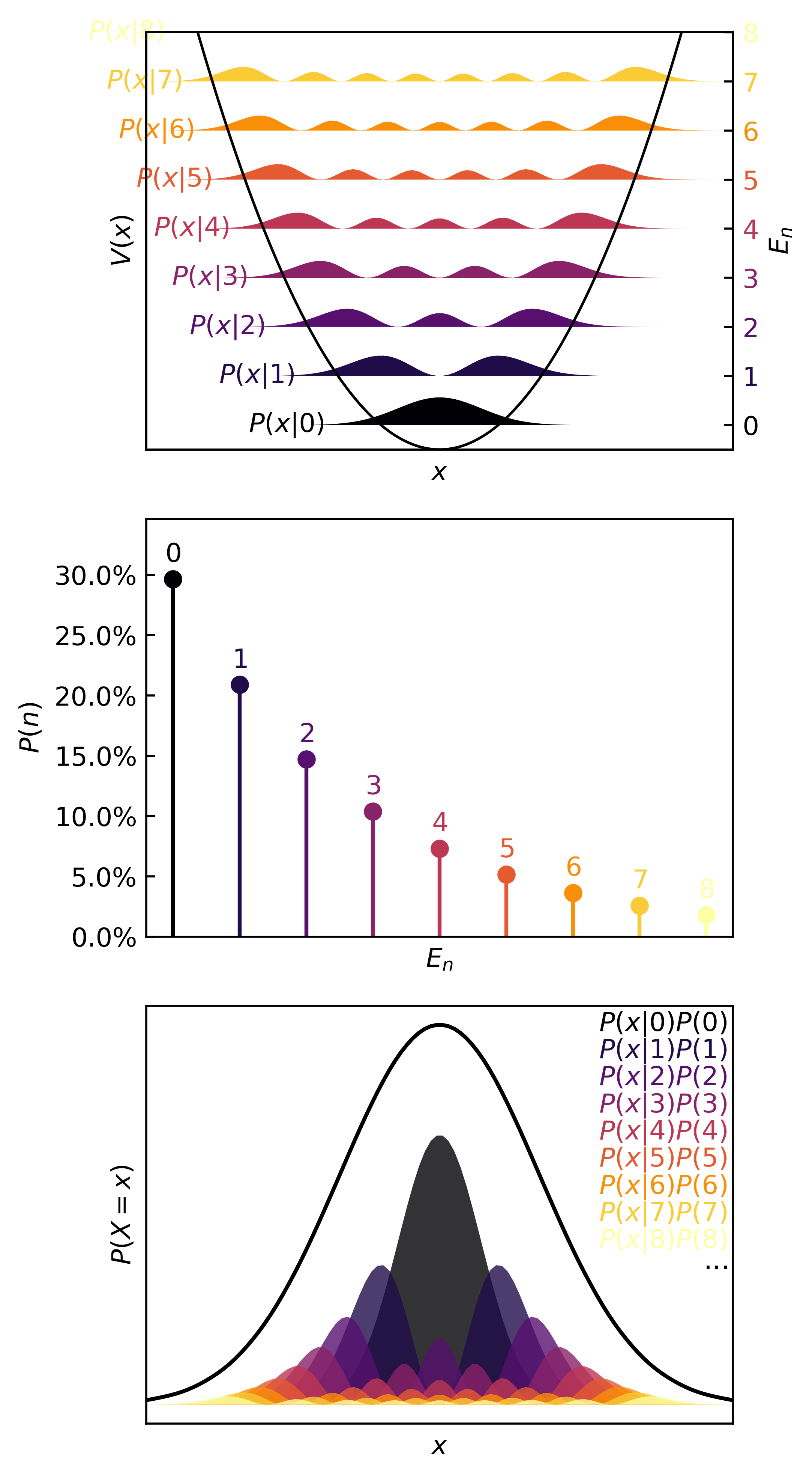
Then we can visualize the quanta, the quantum probability masses, and the continuous distributions in $x$:

>>> plotter(ho, b=0.35)

Now we have all the parts to learn more complicated quanta by approximating $V(x)$ and based on data. For example, we can generate 1-D slices/margins of data from electronic structure software (like Q-Chem, where I worked in grad school), and then fit the data to a polynomial using a linear regression model.

$$V (x) \,=\, \sum_{j=0} c_j x^{j}$$

nn = torch.nn
class Polynomial(nn.Module):
    def __init__(self, order=8):
        super().__init__()
        self.c = torch.nn.Parameter(torch.zeros(order), requires_grad=True)
    
    def forward(self, x):
        y = 0.
        for i,c in enumerate(self.c):
            y += c*torch.pow(x, i)
        return y

Then we can define this potential in a quantum model in the PolynomialBasis class, train it on generated data, and update the $H$ matrix in the same basis like this:

$$\begin{aligned} \bra{m} \hat{H} \ket{n} &\,=\, \bra{m} \underbrace{\frac{1}{2} \hat{\nabla}^2 + \hat{V}_\text{HO}}_{\hat{H}_\text{HO}} - \hat{V}_\text{HO} + \hat{V} \ket{n} \\ &\,=\,\left(n + \frac{1}{2}\right)\delta_{mn} + \int \text{d}{x} \,\,\, \psi_m^*({x}) \left[- \frac{1}{2} x^2 + \sum_{j=0} c_j x^j \right]\,\psi_n({x}) \end{aligned}$$

A matrix mechanical trick is to use a matrix operator $\hat{x}$ that relates the position basis to the HO basis. Then we won’t have to crunch all those integrals. The math behind this idea dips into some complex topics like creation & annihilation, so just trust me bro:

$$\bra{m}\hat{x}\ket{n\pm 1} \,=\, \frac{1}{2}\sqrt{m+n+1}$$

$$\mathbf{X}_{mn} \,=\, \frac{1}{2}\sqrt{m+n+1}\,\, \delta_{\left|{m-n}\right|,1}$$

So for each step $-\nabla \log p(c_j\vert x)$ in the optimization, we can update $\mathbf{H}$ & diagonalize to find the eigenvalues & the system’s expectations

$$\mathbf{H} \,=\, \mathbf{H}_{\text{HO}} - \frac{1}{2} \mathbf{X}^2 + \sum_{j=0} c_j \mathbf{X}^j$$

More code:

class PolyQModel(nn.Module, HarmonicOscillator):
    def __init__(self, potential_model, dim):
        super().__init__()
        super(HarmonicOscillator, self).__init__(dim)
        self.X = self._X2q(dim)
        self._potential = potential_model
        # self.update()
        self.loss_fn = F.mse_loss
    
    def forward(self, x):
        return self._potential(x)

    def potential(self, x):
        return self(x)
    
    def update(self):
        H = self.H_base.clone() - 0.5*self.X@self.X
        for i,coeff in enumerate(self._potential.c):
            H += coeff * torch.matrix_power(self.X, i)
        self.H_matrix = H
    
    @staticmethod
    def _X2q(dim):
        """Second quantization X matrix"""
        n = torch.arange(0, dim-1)
        m = torch.arange(1, dim)
        return 0.5*(torch.diag(torch.sqrt(m+n+1), 1) + torch.diag(torch.sqrt(m+n+1), -1))

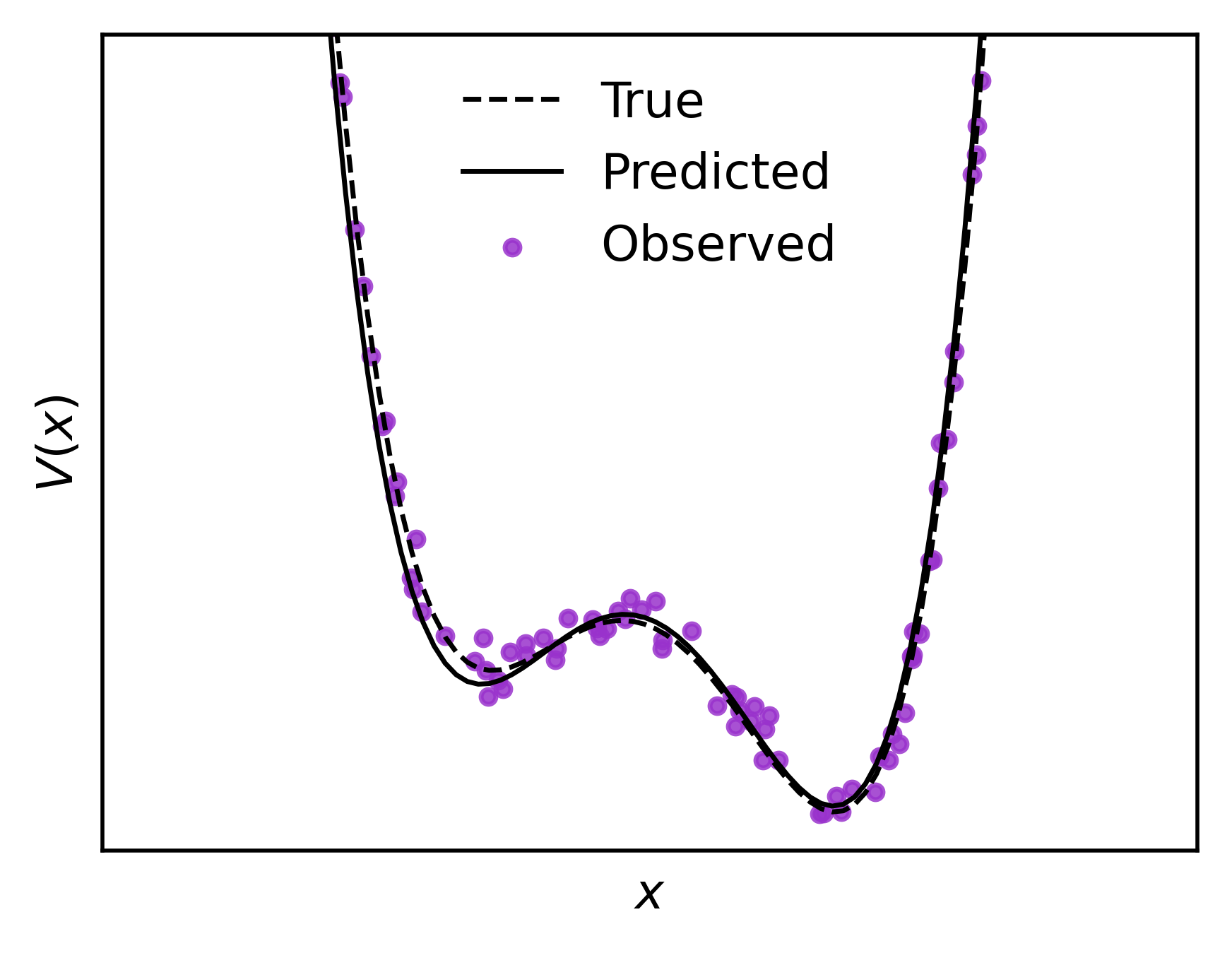
We can see how this model works defining a synthetic $V(x)$ as our “ydata”, and a simple uniformly distributed “xdata”

# Define the "true" potential energy
V = lambda x: x**4 - 5*x**2 + 0.5*x + 6
D = torch.distributions
xdata = D.Uniform(-4, 4).sample((100, 1))
eps = 0.5*torch.randn(xdata.shape)
ydata = V(xdata) + eps

We define our polynomial potential up to power 5, and fit the generated data to the model using the standard optimization cycle with a mean squared error loss function & stochastic gradient descent, updating $\mathbf{H}$ each epoch.

potential = Polynomial(5)
pqmodel = PolyQModel(potential, 16)
cost = nn.MSELoss()
optim = torch.optim.Adam(pqmodel.parameters(), lr=1e-2)
for step in range(100):
    for x,y in zip(xdata, ydata):
        optim.zero_grad()
        pred = pqmodel(x)
        loss = cost(pred, y)
        loss.backward()
        optim.step()
    pqmodel.update()

>>> fit_plotter(pqmodel, (xdata,ydata), true_potential=V)

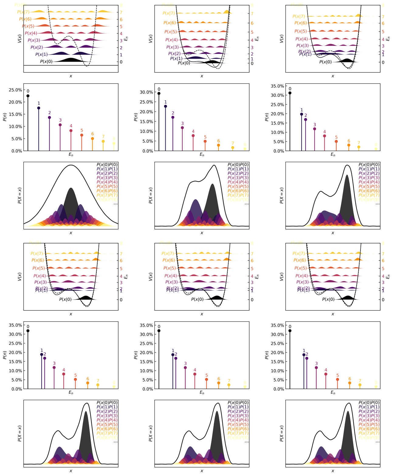
Using the same plotter as before, here’s a gif for the training process. This will allow us to visualize how $X$ is distributed in space, and how $V(x)$ restricts the variable $X$, and how the stochastic gradient descent learns the quanta.

>>> plotter(pqmodel, b=0.25)

In the real (physics) world, this kind of distribution is characteristic of something like a transfer of one atom in one molecule to another molecule, the definition of a chemical reaction. Since atoms are simply too small to isolate, observe, and measure reliably, chemists rely on the observed macroscopic effect of several microscopic events. In statistical terms, only the means of quantities can be observed. These are the expectation, mode, variance, etc.

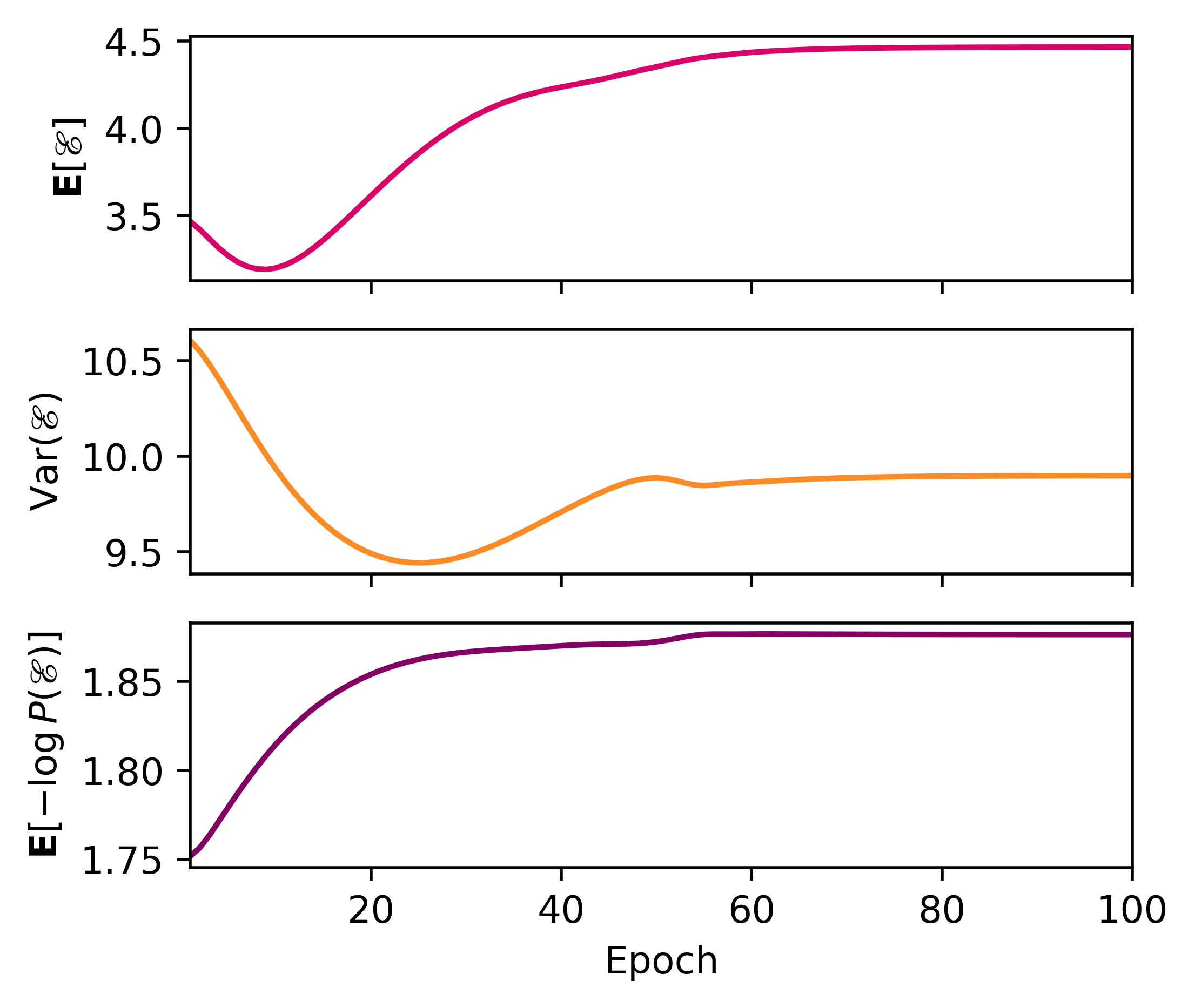
>>> with torch.no_grad():
...    print(qmodel.expectation(b=0.25), qmodel.variance(b=0.25), qmodel.entropy(b=0.25), sep='\n')
...
    tensor(4.4741)
    tensor(10.0515)
    tensor(1.8712)

Connection to Probabilistic ML and conclusion

Obviously we have elements of regression, polynomial fitting, statistics, & linear algebra in this post. But less obviously, this quantum toy model is the foundation for a Bayesian model. That’s because this small model is the ideal a priori estimate to use as a

! prior 😱

on components of a large-dimensional model. In MLspeak, this probabilistic module – trained on a slice of data – can provide probabilistic context to a larger computational model. Such priors regularize model behavior & enable posterior prediction via Markov chain Monte Carlo methods (Hamiltonian Monte Carlo algorithms like NUTS).